The Reservoir Flood Mapping specification 2016 (RFM16), and variants before it, advocate that inundation models are undertaken using a "flat roughness" approach. For a specification that also suggests a use of a 2 m resolution hydraulic grid based 2D model, this seems a bit inappropriate. This is in no way an attack on more detail: using the 2 m LIDAR products for England and Wales is a fantastic idea for inundation modelling and it works very well, however to suggest that fine resolution topography alone will improve our understanding of the flood plain dynamics would be incorrect. Hear me out.
RFM16 suggests a Manning's n value of 0.1, which is accepted by the guidance to be a little on the high side to account for urban areas and wooded areas. A Manning's n value of 0.1 is actually broadly described as follows by Chow, 1959:

• Channels: very weedy reaches, deep pools, or floodways with heavy stand of timber and underbrush
• Flood Plains, Brush: medium to dense brush, in summer
  
• Flood Plains, Trees: heavy stand of timber, a few down trees, little undergrowth, flood stage below branches
  

To suggest that application of these values broadly will help define the hydraulic regime on roadways, open ground and smooth hard surfaces would be optimistic at best. In fact, adopting a 0.1 value as being 'average' is a little dangerous, just because of how 2D surface water equation models account for losses. To explore this, we'll need to look at how roughness is actually considered by a 2D SWE model in a finite volume regime.
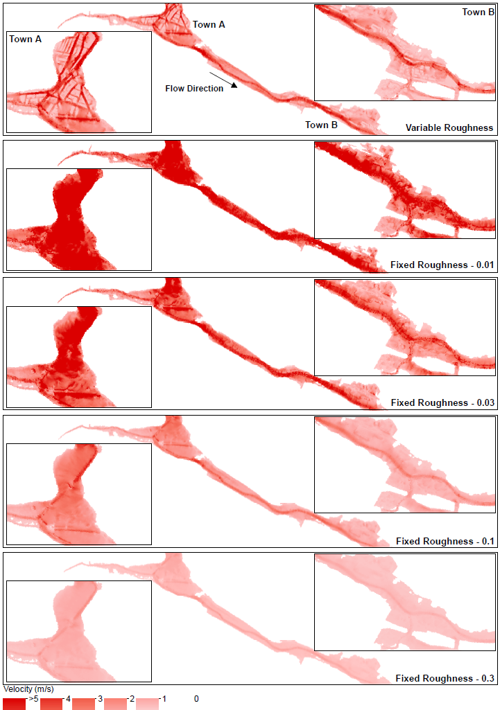
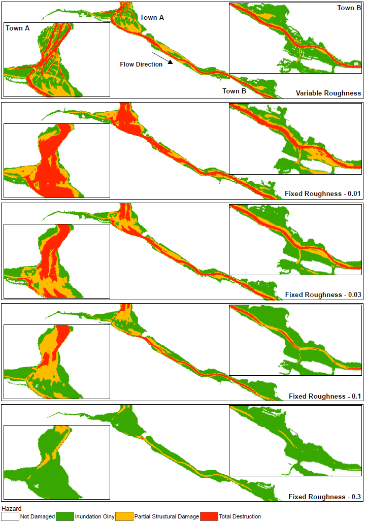
Without quoting the direct transport equations (because it isn't really important) it is important to understand that there are 2 underlying principles of shallow water equation models. The first is mass or volume conservation. This simply states that the volume in any control volume will increase or decrease as a function of the inflow and outflow, plus any effects from 'sources' (i.e. inflows and outflows from the domain which occur within the control volume). Roughness has no direct impact in these equations. It does instead appear in the second underlying principle: momentum conservation.
Momentum conservation can be thought of as the fluid loading. A major component of this, as you may have guessed, is gravity. So if fluid depth is high on one side of the control volume, and fluid depth is low on the other - momentum will load the control volume in the net downstream direction. After this term there is a roughness term, and it looks a bit like this:

Where F is force, V is a velocity vector, of which u and v are the x and y components respectively. H is the height of the fluid in the control volume. Manning's n is used in Lambda as follows:

This tells us a few things. Firstly, if we carry H outside of lambda we retain a negative exponent: this means that in deep water roughness effects are reduced a little bit. This makes sense, since roughness is in effect a measure of the bed shear resistance of the fluid. A greater depth means an increased depth over which shearing can take place. But perhaps the most important thing to consider is Manning's n. Frictional loading is related to n squared.
This means you cannot simply 'take an average value' to account for both rough and smooth values of roughness and expect to develop a good understanding of the resulting hydraulic regime. This is very important especially in dense urban areas where there is a steep gradient in roughnesses between smooth and open roadways, gardens and cultivated parks, and buildings (which can be modelled as high roughness).
We put this to the test in a recent piece of research and demonstrated that while inundation depths are not particularly sensitive to roughness (since they do not play a major part in the volume conservation aspect of SWEs), velocities are.

Velocities are so sensitive to roughness that they significantly distort the Depth Velocity product. This is something that we typically use in the dams industry to score both building damage and fatality rates. This means that by adopting a fixed value, especially of 0.1, you may significantly underestimate the number of fatalities and building damage/third party losses.

We've shown that if you need to take a fixed value of roughness, a value somewhere between 0.035 and 0.1 will be most appropriate, and that 0.1 is too high. Ideally, you want to do a variable roughness model, and there are a number of reasons which suggest that a grid based 2D model might therefore not be the best approach (and that a Flexible Mesh model might instead be more appropriate).

Are you thinking about your dam break assessments, or some other type of rapid inundation model? CCH can help. We are very experienced with this type of modelling and have published works in this field related not only to roughness, but also novel applications of predictive breach models, stochastic and disaggregated life loss models, and fragility based building damage and loss modelling.

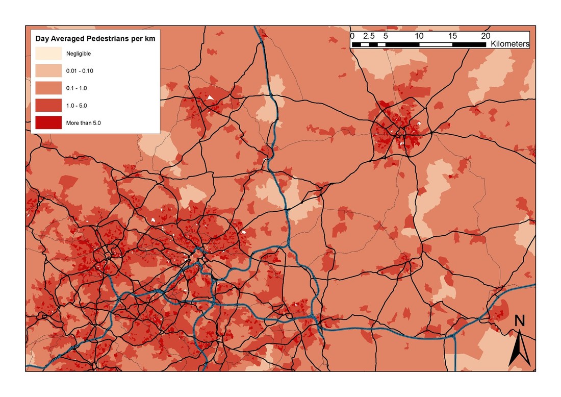
​Have you recently used RARS Table 9.3, or simply omitted transport system users in your PAR calculations? It turns out that you might have underestimated the exposed population at risk.
Ever since the Interim Guide was published in 2004, dam engineers undertaking failure inundation mapping typically tend to calculate the Population At Risk adopting the approach that has been included in the Risk Assessment for Reservoir Safety Management (RARS) Tier 2 methodology. This uses a combination of the number of vehicles a day, the occupancy rate of those vehicles, and the average speed to, broadly speaking, determine a notional PAR per distance of network. Table 9.3 of this document is often referenced in order to determine the population at risk on transport networks. It includes 4 types of network: A Road, Country Lane, Footpath, and Railway.
I would like to stress that, at the time of first publication, Table 9.3 (which was first included in the Interim Guide and its supplementary publications) was the best guidance available. It is only in recent years that adoption of this table has been questionably inappropriate due to advances in simulation techniques and improved data availability.
The underlying data supporting this table has not been updated in a number of years. And furthermore because of the populations assessed for each of these transport networks (i.e. 'A Road' only considers cars) the full PAR value hasn't been calculated. Truth be told, I know of a number of consultants who have, in recent years, dropped assessing transport networks altogether. When asking why they did this, usually the answer that comes back is 'it never seems to make much of a difference'.
As I was embarking on a recent dam failure simulation project, this approach bothered me. 'It never seems to make a difference'. Does this honestly stand up to any form of rigorous scrutiny? I personally doubt it. This is like saying 'we chose not to adopt a method because it gives negligible results' rather than saying 'hmm. This method seems to give very low numbers which might not be realistic, I wonder whether I should investigate further'.
The real reason why I started to question this was because, behind the scenes, I've been developing a coupled, stochastic damage and life loss model for inundation zones (further publications in due course) - and it needs a realistic disaggregated set of PAR values. I noticed on reviewing many shocking survivor videos from a number of tsunamis that, unless a shelter fails, it really is predominantly the exposed populations (i.e. pedestrians, cyclists, car and other vehicle occupants) who are the most at risk from sudden hydraulic loading. To simply adopt a PAR(transport) of 0 doesn't make sense, and it is not what is observed in storm surges, tsunamis, and other very intense flooding events. Further to this survivor videos are often taken from the safety of a rooftop or elevated position (i.e. sheltering populations), and normally the footage focuses on pedestrians or vehicles fleeing the active inundation zone (i.e. exposed populations). You do not need to search websites like YouTube for long to see this demonstrated.
So, with some justification to challenge Table 9.3 in RARS, I considered producing an update. Rather than focus on an arbitrary 500 m inundation zone (as is done in said table), I instead focused on developing generalised PAR values, in the units of people per kilometre. Quickly I discovered a huge wealth of statistical data that is freely available from the Department for Transport. Not only does it give regional and national survey values for annualised average daily flow (AADF) disaggregated by transport mode, but it also has documentation covering average speeds for different classes of vehicles. This is perfect, and off the back of this I very quickly determined the PAR/km for various road classifications on a national level using the following equation

Where PAR(R,C) is the PAR per km for road class R and vehicle class C, n is the annual average daily flow (vehicles per day), o is the average occupancy of the vehicle (people per vehicle) and v is the velocity (m/s). Using the Department for Transport values, you can work this out for each road class, and for different classes of powered vehicles.
It will not, however, tell you how to determine the number of pedestrians on a roadway. This is a much more complicated task, and whilst I give a summary of how I did this in my recent paper 'Calculating the population at risk for transport system users' (Dams and Reservoirs, due for inclusion in Volume 27 Issue 2), it is a method which does not produce values which are easily summarised into a PAR(R,C) format. Whilst I give some notional values, I also detail the method I used to get baseline numbers for various urban and rural areas (I used an area of Yorkshire as a sample since it have a good variety of urban and rural spaces). Generally I found that, as you might expect, pedestrians are more commonly encountered in urban spaces.
This is a different approach, and it uses census data and some assumptions about how (or more specifically, where) walks start and end. If this is something that interests you, I suggest looking into the paper. It allowed me to produce a map like this (for Leeds/Bradford and York):

So what was the major finding? It turns out the Table 9.3 has inadvertently (and through republishing without updates) given values which, in some cases, might be an order of magnitude too small. The paper presents a new table, which brings Table 9.3 back in line with calculated values, but it also includes a more detailed disaggregated (by vehicle class and road type) table for anyone doing more detailed inundation mapping. Additionally, if you are working in a specific region, you can follow the documented method to calculate bespoke PAR values.
The use of Table 9.3 is an example of one of a few bits of guidance that, during initial production, was conceived under the notion that they would be updated once better information became available. Just like Figure 9.1 (fatality rates from RARS) which I am also currently updating, it has instead been adopted as 'the last word' or 'guidance', even though it was never intended for use in extremely detailed studies and is based on little or no validation data. Furthermore, neither of these were designed with point application in mind (2D modelling was not regularly undertaken for inundation models in the late 1990s and early 2000s) - so applying them without at least questioning them would be inappropriate at best, and non-conservative at worst (bear in mind the usual applications for this type of study).
So the next time you find yourself saying 'I can leave this out because it never makes a difference', I urge you to question that way of thinking - and to challenge the source data and assumptions that led you there in the first place.